Disclaimer: This article was originally published on my LinkedIn click here on September 8, 2018.

The code is available HERE: agilajah/multi-armed-bandits.
Introduction
I can’t believe that this is already the 5th instalment of ‘ML.rand() series’. A series in which we can discuss virtually anything about Machine Learning randomly.
I think I am going to break my rule here. Usually, I write each article with a topic that is different from the other so that the reader could jump to whichever part as they please. Unfortunately, I can’t do that for now because starting from this part (and for some subsequent articles), I will be dissecting AlphaGO Zero. This is a great opportunity to finally work out the details and to develop (complete) understanding of two-person zero-sum perfect information games so that I (and you) can completely grok what makes AlphaGoZero tick. To limit the discussion into only one article would be limiting my study and I don’t want to miss out on this opportunity.
There are four major concepts used in AlphaGo Zero: Multi-Armed Bandits & UCB, Minimax & Alpha-Beta Pruning, Policy & Value Functions, and Monte Carlo Tree Search & UCB For Trees. So I planned to write (at least) 4 articles, each dedicated to a particular concept. In addition, there would be one article in which we integrate MCTS and Reinforcement Learning. Finally, we’ll be discussing the AlphaGoZero paper and explore a related paper in the last article. In total, there would be 6 articles for this AlphaGO Zero Edition series. At the risk of failing miserably, I’ll give it a try nonetheless. :D
I assume the reader is familiar with the basic of Python as I’ll write the code in Python to explain some concepts and further aid intuition. Additionally, I hope the reader is comfortable with reading little math equations.
Now, let’s take a look at the following diagram:
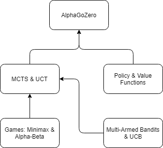
Figure I. Concepts used in AlphaGoZero. Source: Personal Gallery. Adapted from: depthfirstlearning.com
The above diagram depicts the concepts used in AlphaGo Zero. We’ll begin our journey by discussing Multi-Armed Bandits & UCB. I hope you enjoy it.
Without further ado, let’s get started.
NOTE: This article is adapted from my own article about multi-armed bandits problem with epsilon-greedy algorithm which can be found here.
Exploration vs Exploitation
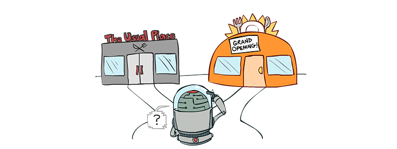
Figure II. I am confused. Source: probyto.com
Decision making is a challenge we all face every day. From choosing a place to eat, to deciding whether or not to invest in some companies; If we go to our favourite restaurant, we will be confident of what we will get. But we will miss the chances of discovering an even better option (with great discounts and stuff).
If we only investing in those already proven companies, maybe we will miss out on opportunities to yield better returns than our current prospects. But by exploring too much, we may won’t make enough profit.
This is what we call by exploration vs exploitation dilemma. When we explore something, we might discover unknown (better) options but we have to sacrifice the other option(s) as well. Although exploration could be a total failure, we’ll gain important lessons from it. On the other hand, when we do some exploitations, we’ll be confident to get what we expected but ended up losing chances that might be better for us.
The thing is, we operate on a daily basis with limited knowledge and little understanding of how the world (or the people, or the markets) works. So, how do we decide when to explore new things and when to take advantage (exploit) of our knowledge on something? After all, we’ve only got so much time in the world and one little mistake (at worst case scenario) could cost you everything. (The hell I was talking about LOL, pardon my language. Let’s move on).
Multi-Armed Bandits Problem

Figure III. Slot machines (‘bandit’ because they steal your money). Source: https://en.wikipedia.org/wiki/Multi-armed_bandit
At its core, Multi-armed bandits problem is all about decision making. It is a framework for understanding the exploitation vs exploration tradeoff. The term “multi-armed bandit” comes from a hypothetical experiment where a person must choose between multiple actions (i.e. slot machines, the “one-armed bandits”), each with an unknown payout.
At each round, we simply pull the arm that has the highest empirical reward estimate up to that point.
Anyway, this problem would be easier if we knew the expected value of each slot machine. We just have to choose a machine with the highest reward at each time. Unfortunately, slot machines don’t work that way. (I know right! the same with life). So we need to estimate the unknown payout from each machine on our own. The key idea is to develop a strategy, which results in the arm with the highest reward probability to be played such that the total reward obtained is maximized.
The algorithms whose goals are to produce a ‘rule’ of selecting a sequence of options that balance exploration and exploitation is called the bandit algorithms. They have now been studied for nearly a century and can be used for configuring web interfaces, dynamic pricing, ad placement, or even clinical trial design. Moreover, believe it or not, (you should though) bandit algorithms are important components of how Monte Carlo Tree Search (MCTS), a key aspect of AlphaGoZero, was originally formalized.
Let’s do some formalism.
Remember that each bandit represents an action. Let’s draw up some notation. Multi-armed bandits can be described as a tuple of <A, R>, where:
- We have K bandits. Let K bandits/actions labeled by the integer {1, 2, 3, … K}. K machines will have reward probabilities {θ1, θ2, θ3, … θk}.
- Each of the k actions has an expected or mean reward called ‘value’ (μ) given that that action is selected at a time step.
- R is a reward function. The reward of action i is a random variable Ri with unknown distribution and unknown expected value μi.
- A is set of actions, each referring to the interaction with one slot machine. We denote the action selected on time step t as At and the corresponding reward as Rt. The ‘value’ of an action a is the expected reward given if it is selected (see point 2 above) and denoted by If action At at the time step t is on the i-th machine, then .
Speaking of reward, you might ask: How are the rewards produced? Well, one option is to draw a reward for action i (Rt) at time t from a fixed distribution (a different reward distribution for each action) and each draw is independent to the other. This setting is called stochastic and it’s what we’ll use here.
If you look at the above definition of multi-armed bandit, it can be seen as a simplified version of Markov Decision Process.
The goal here is to maximize the cumulative reward (over time). Or equivalent to minimize the potential regret or loss by not picking the optimal action (if we know the optimal action).
ϵ-greedy algorithm
Note that we can’t do both exploration and exploitation at the same time. For a specific case, the choosing of whether or not to explore/exploit at a time step t needs to take into account the estimated value for each action, uncertainty, and the remaining step (this one is optional). Several simple methods are available to balance exploration and exploitation such as ϵ-greedy which enforces non-greedy action (exploration) randomly so that the vast majority of the chosen actions would be exploitations. But it takes random explorations with a probability of ϵ occasionally. (Note: We call exploitation as greedy action, and non-greedy action otherwise). However, ϵ-greedy heavily depends on what kind of task that it is trying to solve. If the variance of the reward is small i.e 0, greedy methods (i.e ϵ equals zero; performs greedy actions at all times) might perform better than ϵ-greedy because without even trying to do exploration we’ve already known the real value of a particular action. (duh! it’s 0 variances)
Recall that the true value of an action is the mean reward when that action is selected. One way to estimate this is by averaging the rewards actually received [1]:
A simple bandit algorithm then goes like this [1]:
Initialize, for a = 1 to k: Q(a) <- 0 N(a) <- 0Loop Forever: A <- argmax Q(a) with probability 1-ϵ (this is greedy action selection) OR <- a random action with probability of ϵ R <- bandit(A) N(A) <- N(A) + 1 Q(A) <- Q(A) + (1 / N(A)) [R-Q(A)]The function bandit(A) takes an action and returns a corresponding reward.
OLD CODE: I’ve already implemented ϵ-greedy one and a half years ago, and you can check the walkthrough (Jupyter Notebook) here.
In the walkthrough, you can see that how different value of ϵ affects the performance of the algorithm. As shown in the following figure.
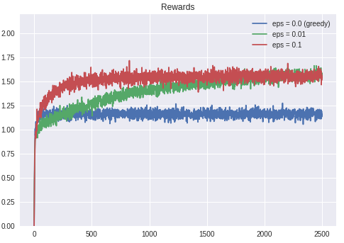
Figure IV. Received reward over time by epsilon-greedy algorithm with different values of epsilon. Source: Personal Gallery.
At first, the ϵ-greedy algorithm with zero ϵ had the best total received reward compared to the other settings, meaning that the reward obtained is very high at the beginning. But over time, it remains at the bottom of the chart; The performance is getting worse in the long run, relative to the others. On the other hand, the ϵ-greedy methods (i.e epsilon != 0) eventually performed better because they continued to explore and improve their chances of recognizing the optimal action. This also reflected by the regrets that the algorithm experienced over time, as shown in Figure V.
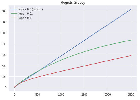
Figure V. Regrets over time for different value of epsilon. Source: Personal Gallery.
Other way to encourage exploration
As we’ve seen in the previous figure, exploration is important. So before talking about another algorithm, I wanted to introduce a simple’r’ way that can be quite effective on stationary problems, but it is far from being a generally useful approach to encouraging exploration. But I think it’s still worth knowing. So let’s do it.
There is something called the bias of initial estimates; All methods that we’ve talked about and will be discussed later is biased by their initial estimate values. Let’s take a look at the following figure to better understand what I meant by the bias of initial estimates.
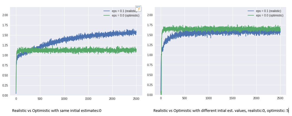
Figure VI. Received rewards of realistic vs optimistic, it is biased by its initial estimate values. Source: Personal Gallery.
Yes, initial estimates can affect the algorithm’s performance for better or worse. Initial action values can also be used as a simple way to ‘encourage’ exploration if you will. That’s why, even with zero epsilon, the algorithm with optimistic initial values (high) could simulate exploration. But this isn’t reliable at all, so we need something better and smarter.
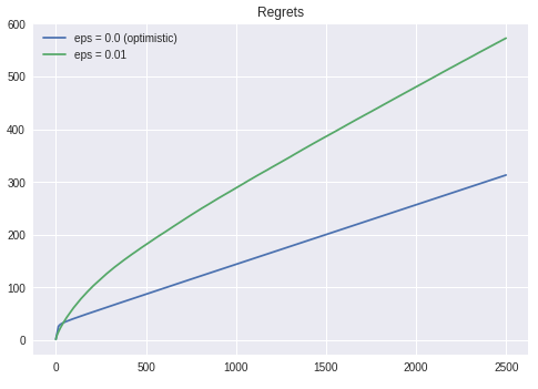
Figure VII. Regrets over time for optimistic vs realistic settings. Source: Personal Gallery.
Upper Confidence Bound
Exploration is needed because there is always uncertainty about the accuracy of the action-value estimates[1]. If we think about it, the way we do explorations can be divided into three ways:
- No exploration (naive)
- Exploration at random (like epsilon-greedy algorithm does)
- Smart Exploration (how? here’s how)
We’ve seen that no exploration at all is bad, and randomly exploring the arms would make us end up revisiting bad actions which we have confirmed in the past. We have two options to remedy this problem though. First, decrease the value of epsilon in time. Second is to explore deterministically by favouring non-greedy actions with the strong potential to be optimal. In other words, we prefer actions for which we haven’t had a confident value estimation yet.
It would be better to select among the non-greedy actions according to their potential for actually being optimal, taking into account both how close their estimates are to being maximal and the uncertainties in those estimates. - Sutton & Barto, Reinforcement Learning
So what we do is to optimistically guess the expected payoff of each action, and pick the action with the highest guess. It is based on the optimism in the face of uncertainty; you choose your actions as if the environment (in this case bandit) is as nice as is plausibly possible [3] or to be more concrete: treating arms which have been played less as more uncertain (and thus plausibly better) than arms that have been played frequently.
The balance of the exploration and exploitation in UCB goes like this: The optimistic guess will decrease if we wrongly guessed the expected payoff so we’ll be compelled to choose other actions; Otherwise we’ll exploit an action if guessed well with little regret.
This optimism comes in the form of Upper Confidence Bound (UCB) of the reward value of an action a: Ut(a). In other words, we want to know with high probability that the true expected payoff of an action is less than our prescribed upper bound :
The upper bound Ut(a) is a function of how many times this action has been selected so far Nt(a) and the larger the Nt(a), the smaller the bound Ut(a). At intuitive level, this term helps us avoid always playing the same arm without checking out other arms. In UCB algorithm, we always select the greediest action to maximize the upper confidence bound:
We need an upper confidence bound to describe the largest plausible mean of each arm.
How to estimate the upper confidence bound?
With the help of Hoeffding inequality we can estimate the upper confidence bound. Suppose X1, X2, … Xt be i.i.d (independent and identically distributed) random variables and they are all bounded by the interval [0, 1]. After doing some magic, we obtained Ut(a) and we have:
Kidding. Alright, let’s start over, if you insisted.
So we have t i.i.d random variables (X1, X2, … Xt) that are bounded by the interval [0, 1], right. The expected values are μi. X is the average of the sum of every Xi and μ = E(X) = the average of the sum of expected values. Recall that Xi is the payoff variable for a single action j. So variable X is the average payoff for action j over all the times we’ve selected it. The Hoeffding inequality gives an exponential upper bound on the probability that the value of deviates from its mean.
See? It’s kinda hard to read. Especially for me. That’s why I skipped over the details. But you insisted. LOL.
Let’s continue. For a given action a, let us consider:
- rt(a) as the random variables (of reward/payoff).
- Q(a) as the true mean.
- Qt(a) is the sample mean.
- u as the upper confidence bound, u = Ut(a).
Then we have:
Recall that we want to know with high probability that the true expected payoff of an action is less than our prescribed upper bound; We want to pick a bound so that the true mean is below the sample mean + the upper confidence bound with high confidence [6].
It means that should be a small probability. Let’s say it’s p. So:
Thus,
Yeah, that’s how you get the Ut(a). Finally, we have:
UCB1 Algorithm
UCB1 is an algorithm proposed by (Auer et al 2002) for the multi-armed bandit that achieves regret that grows only logarithmically with the number of actions taken. (You guys should definitely check the original paper HERE and refer to this note for the analysis). One heuristic is to reduce the threshold p in time, as we want to make more confident bound estimation with more rewards observed. [6], Set we get:
and,
Thus,
So, that’s how you derive the equation. Intuitively, then the algorithm goes like this[2]:
![UCB1 Algorithm. Source: [2] UCB1 Algorithm. Source: [2]](/assets/2018/september/random-ml-5-10.png)
Implementation
I implemented the above algorithms (including the epsilon greedy) HERE: agilajah/multi-armed-bandits. Note that it’s only a ‘toy problem’ for the sake of aiding intuition. I’m aware that this isn’t at all a proper implementation in terms of the code quality, lol. It’s because I wanted to minimize my effort, so I was just using my old code and added UCB1 algorithm in it without huge refactoring. But I hope that you could grasp what I’ve been talking about by looking at that code.
As expected, UCB1 produces better result. It’s also ‘experienced’ lowest regrets (at least if we compare it to epsilon greedy at this scenario). I feel that ‘experienced’ is not the right word for this. But whatever lol
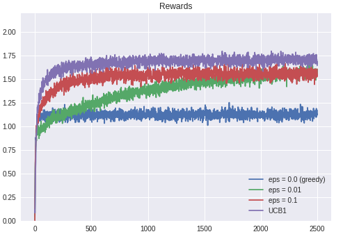
Figure VIII. Received rewards by UCB1 algorithm vs Epsilon Greedy with various epsilon values. Source: Personal Gallery.
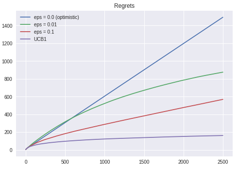
Figure VIII. Forget regret, or life is yours to miss. Source: Personal Gallery.
Final Remarks
So I guess that’s it for the first part of Understanding AlphaGo Zero series. It’s a long post, but worth to read (I think). We’ve learnt how important an exploration is. The information that we get from an exploration is really valuable in order for us (or an agent) to be able to decide things with minimal regret. OK I don’t what I am talking about, so I think we should end this article here. If you catch any error, please do contact me via LinkedIn message, or email me at febiagil@gmail.com. Stay tuned for the next part.
References
-
[0] Auer, P., Cesa-Bianchi, N., & Fischer, P. (2002). Finite-time analysis of the multiarmed bandit problem. Machine learning, 47(2-3), 235-256.
-
[1] Sutton, R. S., & Barto, A. G. (2018). Reinforcement learning: An introduction, second edition (DRAFT). http://incompleteideas.net/book/bookdraft2018jan1.pdf
-
[2] https://jeremykun.com/2013/10/28/optimism-in-the-face-of-uncertainty-the-ucb1-algorithm/
-
[3] http://banditalgs.com/2016/09/18/the-upper-confidence-bound-algorithm/
-
[5] Burtini, G., Loeppky, J., & Lawrence, R. (2015). A survey of online experiment design with the stochastic multi-armed bandit. arXiv preprint arXiv:1510.00757.