Disclaimer: This article was originally published on my LinkedIn (click here) on May 6, 2018.
Note: the primary goal of these series that I’ve been working on is simply to keep a record of the papers I’ve read and things I learned along the way. If you find anything inaccurate, kindly let me know.
TLDR; We want to make an optimizer as general as possible by replacing hand-designed update rules with a learned update rule, which is modelled by an RNN. Now, you might ask why…

The answer lies with the rest of this article :)
Introduction
Welcome to the second instalment of ML.rand(), a brand-new series where we can discuss virtually anything about Machine Learning randomly.
In a previous article, we’ve learned about how to train a neural network ‘without’ backpropagation. Now, we’re going to learn about how to teach a machine to learn how to learn (It’s kind of confusing, but bear with me. :D ) from a paper which was released in 2016 by a team of researchers from Google DeepMind, University of Oxford, and Canadian Institute for Advanced Research named: Learning to learn by gradient descent by gradient descent.
Is that a typo?
Umm, no it isn’t. Such a cool title, right?
So, before we begin, I would like to invite you all to take a moment to reflect on how we usually formulate a machine learning task. If you think carefully about it, a task in machine learning is just an optimization problem of which we want to find the minimizer of a function f(θ). You could really call machine learning as function learning, btw. But nah.. that doesn’t sound cool.
We usually perform a sequence of updates to minimize the objective function f(θ) with gradient descent as follows:

But sometimes, vanilla gradient descent isn’t enough to do the job and perform rather poorly for some tasks because of its nature. That’s why we’re usually playing around with a tailored update rule for a particular task (or a class of problems). Moreover, we have lots of optimization methods including Momentum, ADAM, and RMSProp. It means that we have a lot of options, and we do get to choose.
Those task-specific optimizers are designed to exploit structure in their problems of interest. Thus, they usually perform quite good, as suggested in No Free Lunch Theorems for Optimization. The thing is, they will potentially perform poorly on problems outside of that scope[1].
What we want is, of course, an update rule that performs well in any tasks, aren’t we? But, are we capable of crafting such a thing? How advanced are we earthlings?
Interestingly, the authors took a different way and proposed a different method. In Learning to learn by gradient descent by gradient descent paper, the authors instead tried to replace those hand-design update rules with a learned update rule called optimizer g which was modelled using an RNN. So, it gives us:

And… it worked. Kaboom.
Wait, what?
Back in the day, we designed a learning algorithm by looking at the problem’s properties. But as we discussed earlier, these hand-crafted learning algorithms are too specific. Moreover, this is where training a neural net becomes more of an art than a science as there are so many possible optimizers and optimization settings (hyper-parameters).
So, how we address this ‘problem’? by magic, really.
Basically, the authors aimed at producing a method to craft a learning algorithm that performs well in a particular optimization problem, automatically: Learning to learn. People called this kind of thing as Meta-learning. They do it by using a Recurrent Neural Networks instead of standard optimizers such as ADAM, RMSProp, etc.
Gone are the days of hand-crafting learning algorithms.
OK. How does it work?
Remember that this work has something to do with learning to learn with a recurrent neural network. Fun fact: gradient descent can be thought of as a mini-RNN because it’s fundamentally a sequence of updates. Our goal now is to train an RNN to replace the optimizer part of a neural network.
So, the idea is to use a separate network that functions using the main function f itself and the parameter of the optimizer theta.
The loss function defined as follows:

Where f is the main function, θ* is the optimizee parameters, and φ is the optimizer parameters. Our original loss function above depends only on the final optimizee parameter value. In order to train the optimizer it will be more effective to have an objective function that depends on the entire trajectory of the optimization, for some horizon T:
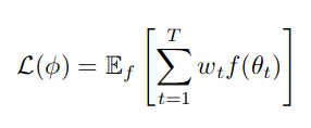
Note: we’re just going to weigh everything with 1 at each timestep.
And we have these following operations:
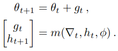
Including ∇t = ∇θf(θt) which is the gradients of f (optimizee) with respect to optimizee parameters at time t. Here, m is our RNN network and we’ll call it the optimizer where gt is the update it outputs at time t, ht is its state at time t. And remember, φ is the optimizer parameters. In layman’s term:
The loss of the optimizer is the sum of the losses of the optimizee as it learns.
Look at the following diagram which depicts the flow of the gradients. The dashed line indicates that the gradient doesn’t flow there.
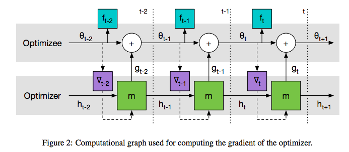
This allows us to state that the gradients of f with respect to to theta at time t are independent of the optimizee’s parameters.
Hmm, easy peasy lemon squeezy.
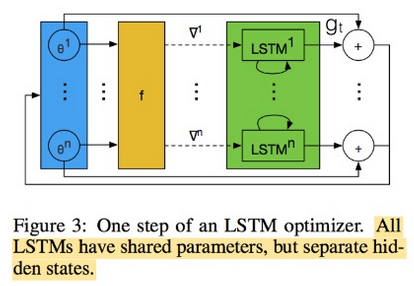
It sounds ‘easy’ in some sense, but also comes with a challenge: the RNN has a lot of parameters. The authors employed a special type of RNN called LSTM but it’s pretty much the same in this matter.
Each cell in the LSTM has four components: the cell weights, the input gate, the forget gate, and the output gate. Each component has weights associated with all of its input from the previous layer, plus input from the previous time step. The number of LSTM parameters, taking input vectors of size m and giving output vectors of size n is:
But if our LSTM model has bias(es), it would be:
So, we’re talking about tens of thousand parameters here. this is a problem in and of itself.
Luckily, the authors came up with a solution. They implemented the network based on coordinatewise network architecture which can be summed up by the following figure:
Results
In their paper, the authors conducted experiments around 4 problems: quadratic function, MNIST, CIFAR-10, and Neural Art. In the following figure, we’ll see that learned optimizers outperform hand-crafted optimizers.

Go check the original paper to find out more.
Final Thoughts
This paper explores the new direction of learning the optimization method itself and is quite interesting as it can potentially address optimization to problems that have not done well with standard approaches. I expect meta-learning to become increasingly more important.
The most important thing is, it works. But I have a slight problem with its scalability as the experiments in the paper are very small. However, I’d like to see more of what it can do.
References
-
[1] Andrychowicz, M., Denil, M., Gomez, S., Hoffman, M. W., Pfau, D., Schaul, T., & de Freitas, N. (2016). Learning to learn by gradient descent by gradient descent. In Advances in Neural Information Processing Systems (pp. 3981-3989).